
Advise the planning department on ways to improve the quantity and quality of trees in Manhattan.
The urban design team believes tree size (using trunk diameter as a proxy for size) and health are the most desirable characteristics of city trees.
Toggle to show summary or use the link to go to the section for more detail
Note: This does not include the "park-cemetery-etc-Manhattan" neighbourhood for which no tree data is provided.
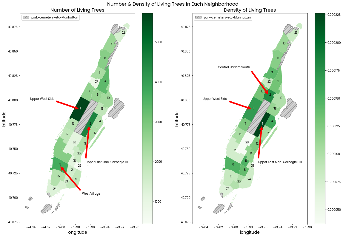
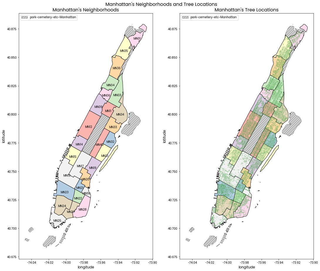
Image attributions can be found at the end of the notebook.
# IMPORTS ==============================================================
import pandas as pd
import geopandas as gpd
import matplotlib.pyplot as plt
import seaborn as sns
import numpy as np
from scipy import stats

import src.style # A file which helps me style all the plots more consistently
The team has provided access to the 2015 tree census and geographical information on New York City neighborhoods (trees, neighborhoods):
Tree census and neighborhood information from the City of New York NYC Open Data.
# READ TREES CSV & PRINT BASIC FACTS ===================================
trees = pd.read_csv('data/trees.csv')
print("Latitude Range:", trees.latitude.min(), trees.latitude.max())
print("Longitude Range:", trees.longitude.min(), trees.longitude.max())
print("Duplicated tree_id:", trees.tree_id.value_counts().max()>2)
print("Number of trees:", len(trees), trees.status.value_counts().to_dict())
print("Number of unique species of tree:")
trees.head(1)
Latitude Range: 40.70178954 40.87305363
Longitude Range: -74.01836049 -73.91120169
Duplicated tree_id: False
Number of trees: 64229 {'Alive': 62427, 'Dead': 1802}
Number of unique species of tree:
| tree_id | tree_dbh | curb_loc | spc_common | status | health | root_stone | root_grate | root_other | trunk_wire | trnk_light | trnk_other | brch_light | brch_shoe | brch_other | postcode | nta | nta_name | latitude | longitude | |
|---|---|---|---|---|---|---|---|---|---|---|---|---|---|---|---|---|---|---|---|---|
| 0 | 190422 | 11 | OnCurb | honeylocust | Alive | Good | No | No | No | No | No | No | No | No | No | 10023 | MN14 | Lincoln Square | 40.770046 | -73.98495 |
# READ NTA SHP DATA & PRINT BASIC FACTS ================================
neighborhoods = gpd.read_file('data/nta.shp')
print("Number of Manhattan neighbourhoods:", neighborhoods[neighborhoods["boroname"]=="Manhattan"]["ntaname"].nunique())
print(
    "No trees in the following neighborhoods of Manhattan:",
    set(neighborhoods[neighborhoods["boroname"]=="Manhattan"]["ntaname"].unique()) - set(trees["nta_name"].unique())
)

neighborhoods['point'] = neighborhoods['geometry'].apply(lambda x: x.centroid.coords[0])
neighborhoods.head(1)
Number of Manhattan neighbourhoods: 29
No trees in the following neighborhoods of Manhattan: {'park-cemetery-etc-Manhattan'}
| borocode | boroname | countyfips | ntacode | ntaname | shape_area | shape_leng | geometry | point | |
|---|---|---|---|---|---|---|---|---|---|
| 0 | 3.0 | Brooklyn | 047 | BK43 | Midwood | 3.579964e+07 | 27996.591274 | POLYGON ((-73.94733 40.62917, -73.94687 40.626... | (-73.95682460579987, 40.620924048798294) |
Oberservations from the data
Consequently...
print(
    "Proportion of trees Alive/Dead:",
    (trees["status"].value_counts() / len(trees)).round(3).to_dict()
)

print(
    "Any missing values for living trees?",
    trees[trees.status == "Alive"].isna().any().any()
)

print("The only dead tree where 'spc_common' is given:")
trees[(trees["status"]=="Dead") & (~trees["spc_common"].isna())]
Proportion of trees Alive/Dead: {'Alive': 0.972, 'Dead': 0.028}
Any missing values for living trees? False
The only dead tree where 'spc_common' is given:
| tree_id | tree_dbh | curb_loc | spc_common | status | health | root_stone | root_grate | root_other | trunk_wire | trnk_light | trnk_other | brch_light | brch_shoe | brch_other | postcode | nta | nta_name | latitude | longitude | |
|---|---|---|---|---|---|---|---|---|---|---|---|---|---|---|---|---|---|---|---|---|
| 28539 | 473703 | 12 | OffsetFromCurb | honeylocust | Dead | NaN | No | No | No | No | No | No | No | No | No | 10002 | MN28 | Lower East Side | 40.710384 | -73.988208 |
print("Value proportions for some categorical columns of `trees`:")

props = pd.DataFrame()
props["Status=Any"] = trees.fillna("NAN").drop(columns=["spc_common", "tree_id", "tree_dbh", "postcode", "nta", "nta_name", "longitude", "latitude"]) \
    .apply(lambda s: (s.value_counts() / len(s)).round(3).to_dict(), axis=0)
props["Status=Dead"] = trees[trees.status == "Dead"].fillna("NAN").drop(columns=["spc_common", "tree_id", "tree_dbh", "postcode", "nta", "nta_name", "longitude", "latitude"]) \
    .apply(lambda s: (s.value_counts() / len(s)).round(3).to_dict(), axis=0)

pd.options.display.max_colwidth = None
props
Value proportions for some categorical columns of `trees`:
| Status=Any | Status=Dead | |
|---|---|---|
| curb_loc | {'OnCurb': 0.933, 'OffsetFromCurb': 0.067} | {'OnCurb': 0.956, 'OffsetFromCurb': 0.044} |
| status | {'Alive': 0.972, 'Dead': 0.028} | {'Dead': 1.0} |
| health | {'Good': 0.737, 'Fair': 0.178, 'Poor': 0.056, 'NAN': 0.028} | {'NAN': 1.0} |
| root_stone | {'No': 0.804, 'Yes': 0.196} | {'No': 1.0} |
| root_grate | {'No': 0.961, 'Yes': 0.039} | {'No': 1.0} |
| root_other | {'No': 0.922, 'Yes': 0.078} | {'No': 1.0} |
| trunk_wire | {'No': 0.986, 'Yes': 0.014} | {'No': 1.0} |
| trnk_light | {'No': 0.995, 'Yes': 0.005} | {'No': 1.0} |
| trnk_other | {'No': 0.913, 'Yes': 0.087} | {'No': 1.0} |
| brch_light | {'No': 0.986, 'Yes': 0.014} | {'No': 1.0} |
| brch_shoe | {'No': 0.999, 'Yes': 0.001} | {'No': 1.0} |
| brch_other | {'No': 0.898, 'Yes': 0.102} | {'No': 1.0} |
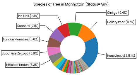
Pie-chart: The proportions of trees belonging to each species. The most common species are labelled with their common name and percentage.
# PLOT PIE CHART OF TREE COUNTS ========================================

def plot_tree_counts(data, num_labelled=8):
    counts = data["spc_common"].value_counts().to_frame("count") \
        .reset_index().rename(columns={"index": "spc_common"})
    counts["percent"] = counts["count"] / counts["count"].sum()
    counts["label"] = counts["spc_common"].str.title() + counts["percent"].apply(lambda x: f" ({x:.1%})")

    fig, ax = plt.subplots(1, 1)
    wedges, texts = ax.pie(counts["count"], wedgeprops=dict(width=0.5), startangle=-50)

    bbox_props = dict(boxstyle="square,pad=0.3", fc="w", ec="k", lw=0.72)
    kw = dict(arrowprops=dict(arrowstyle="-"),
            bbox=bbox_props, zorder=0, va="center")

    for i, p in enumerate(wedges[:num_labelled]):
        ang = (p.theta2 - p.theta1)/2. + p.theta1
        y = np.sin(np.deg2rad(ang))
        x = np.cos(np.deg2rad(ang))
        horizontalalignment = {-1: "right", 1: "left"}[int(np.sign(x))]
        connectionstyle = "angle,angleA=0,angleB={}".format(ang)
        kw["arrowprops"].update({"connectionstyle": connectionstyle})
        ax.annotate(counts["label"].loc[i], xy=(x, y), xytext=(1.35*np.sign(x), 1.4*y),
                    horizontalalignment=horizontalalignment, **kw)

    return fig, ax

fig, ax = plot_tree_counts(trees)
fig.suptitle("Species of Tree in Manhattan (Status=Any)", y=1.05);
# fig.savefig("figs/species.png", facecolor="white", bbox_inches="tight");
plt.close()
Left: A map of Manhattan's neighborhoods colored by its total count of living trees. Darker color means more trees by total count.
Right: A map of Manhattan's neighborhoods colored by its density of living trees. Darker color means more trees per area of neighborhood.
The number in each neighborhood is its ranking. Where "1" indicates the state had the most trees by total count or per area. The top 3 neighborhoods in each subplot are also labelled with red arrows and their names.
The grey hatched areas are of the "park-cemetery-etc-Manhattan" neighborhood which does not contain any trees in the data provided.
# SETUP FOR FOLLOWING GEOPANDAS MAP PLOTS ==============================
# SOME GEOPANDAS PLOTTING KWARGS ---------------------------------------
annot_kwargs = dict(
    textcoords='axes fraction',
    arrowprops=dict(color='red', shrink=0.05),
    horizontalalignment='right',
    verticalalignment='top',
    xycoords='data'
)
missing_kwds = {
    "facecolor": "lightgrey",
    "edgecolor": "grey",
    "hatch": "///",
}

# A TWO PANEL LAYOUT I WILL USE REPEATEDLY -----------------------------
def dual_layout(suptitle, titles, figsize=(18, 20), y=0.82):
    fig, ax = plt.subplots(1, 2, figsize=(18, 20))
    fig.suptitle(suptitle, y=y, fontsize=16)
    for i, a in enumerate(ax):
        a.set_title(titles[i], fontsize=16)
        a.set_xlabel("longitude", fontsize=12)
        a.set_ylabel("latitude", fontsize=12)
    return fig, ax

# SOME OBJECTS TO ENABLE CUSTOM LEGENDS --------------------------------
import matplotlib.patches as mpatches
class AnyObject(object):
    pass

class AnyObjectHandler(object):
    def legend_artist(self, legend, orig_handle, fontsize, handlebox):
        x0, y0 = handlebox.xdescent, handlebox.ydescent
        width, height = handlebox.width, handlebox.height
        patch = mpatches.Rectangle([x0, y0], width, height, lw=1,
                                   transform=handlebox.get_transform(),
                                   **missing_kwds)
        handlebox.add_artist(patch)
        return patch
# PLOTTING NEIGHBORHOOD TREE COUNTS AND DENSITIES ======================
# PREP DATA ------------------------------------------------------------
d = pd.DataFrame()
d["Alive"] = trees[trees["status"]=="Alive"]["nta_name"].value_counts()
d["Dead"] = trees[trees["status"]=="Dead"]["nta_name"].value_counts()
d = d.reset_index()
d.columns = ["nta_name", "alive", "dead"]
d["total"] = d["alive"] + d["dead"]
d["survival"] = d["alive"] / d["total"]
d = d.append(pd.Series({"nta_name": 'park-cemetery-etc-Manhattan'}), ignore_index=True) #.fillna(0)
# print(d.head())

man = pd.merge(neighborhoods[neighborhoods["boroname"]=="Manhattan"], d, left_on="ntaname", right_on="nta_name")
assert man["boroname"].nunique() == 1
# print(man.head())

man["alive/area"] = man["alive"].divide(man["shape_area"])
man["alive_rank"] = man["alive"].rank(ascending=False)
man["alive/area_rank"] = man["alive/area"].rank(ascending=False)

# CREATE CANVAS --------------------------------------------------------
fig, ax = plt.subplots(1, 2, figsize=(19, 13))
fig.suptitle("Number & Density of Living Trees in Each Neighborhood", y=0.92, fontsize=16)
ax[0].set_title("Number of Living Trees", fontsize=16)
ax[1].set_title("Density of Living Trees", fontsize=16)
ax[0].set_xlabel("longitude", fontsize=14)
ax[0].set_ylabel("latitude", fontsize=14)
ax[1].set_xlabel("longitude", fontsize=14)
ax[1].set_ylabel("latitude", fontsize=14)

# PLOT MAP -------------------------------------------------------------
man.plot("alive", cmap="Greens", ax=ax[0], legend=True)
man.plot("alive/area", cmap="Greens", ax=ax[1], legend=True)
man[man.nta_name=="park-cemetery-etc-Manhattan"].plot(ax=ax[0], **missing_kwds)
man[man.nta_name=="park-cemetery-etc-Manhattan"].plot(ax=ax[1], **missing_kwds)

# ANNOTATIONS ----------------------------------------------------------
for i, row in man.iterrows():
    if row["nta_name"] != 'park-cemetery-etc-Manhattan':
        ax[0].annotate(int(row["alive_rank"]), xy=row["point"], color="white" if row["alive_rank"]==1 else "black")
        ax[1].annotate(int(row["alive/area_rank"]), xy=row["point"], color="white" if row["alive/area_rank"]==1 else "black")

# Annotate top neighbourhoods
man = man.sort_values("alive", ascending=False)
ax[0].annotate(man.iloc[0]["ntaname"], xy=man.iloc[0]["point"], xytext=(0.3, 0.6), **annot_kwargs)
ax[0].annotate(man.iloc[1]["ntaname"], xy=man.iloc[1]["point"], xytext=(0.95, 0.3), **annot_kwargs)
ax[0].annotate(man.iloc[2]["ntaname"], xy=man.iloc[2]["point"], xytext=(0.7, 0.15), **annot_kwargs)

man = man.sort_values("alive/area", ascending=False)
ax[1].annotate(man.iloc[0]["ntaname"], xy=man.iloc[0]["point"], xytext=(0.95, 0.3), **annot_kwargs)
ax[1].annotate(man.iloc[1]["ntaname"], xy=man.iloc[1]["point"], xytext=(0.5, 0.75), **annot_kwargs)
ax[1].annotate(man.iloc[2]["ntaname"], xy=man.iloc[2]["point"], xytext=(0.3, 0.6), **annot_kwargs)

man[["ntaname", "alive", "alive_rank", "alive/area", "alive/area_rank"]].to_csv("results/density.csv", index=False)

# LEGEND ---------------------------------------------------------------
ax[0].legend([AnyObject()], ['park-cemetery-etc-Manhattan'],
           handler_map={AnyObject: AnyObjectHandler()}, loc="upper left")
ax[1].legend([AnyObject()], ['park-cemetery-etc-Manhattan'],
           handler_map={AnyObject: AnyObjectHandler()}, loc="upper left")

# fig.savefig("figs/density.png", bbox_inches="tight", facecolor="white")
plt.close()
Left: A map of Manhattan's neighborhoods with neighborhood codes labelled.
Right: A map of Manhattan's neighborhoods with green points showing locations of trees.
Neighborhood code and tree locations are shown in side by side subplots because having them superimposed on the same plot makes it difficult to see some tree locations.
The grey hatched areas are of the "park-cemetery-etc-Manhattan" neighborhood which does not contain any trees in the data provided.
See Appendix B for a map of dead tree locations and another version using kernel density estimation to show the distribution of trees.
# SCATTERPLOT ON MAP SHOWING LIVING TREE LOCATIONS =====================
# CREATE CANVAS --------------------------------------------------------
fig, ax = dual_layout(
    suptitle="Manhattan's Neighborhoods and Tree Locations",
    titles=("Manhattan's Neighborhoods", "Manhattan's Tree Locations")
)

# PLOT MAP -------------------------------------------------------------
man[man.nta_name=="park-cemetery-etc-Manhattan"].plot(ax=ax[0], **missing_kwds)
man[man.nta_name=="park-cemetery-etc-Manhattan"].plot(ax=ax[1], **missing_kwds)
man.dropna().plot(ax=ax[0], cmap="Pastel1", edgecolor="black")
man.dropna().plot(ax=ax[1], cmap="Pastel1", edgecolor="black")

sns.scatterplot(data=trees, x="longitude", y="latitude", ax=ax[1],
                s=1, alpha=0.3,
                # hue="status",
                color="green"
                )

# ANNOTATIONS ----------------------------------------------------------
for i, row in man.dropna().iterrows():
    ax[0].annotate(row["ntacode"], xy=row["point"],
        horizontalalignment="center", fontsize=10,
        verticalalignment="top")

# LEGEND ---------------------------------------------------------------
ax[0].legend([AnyObject()], ['park-cemetery-etc-Manhattan'],
           handler_map={AnyObject: AnyObjectHandler()}, loc="upper left")
ax[1].legend([AnyObject()], ['park-cemetery-etc-Manhattan'],
           handler_map={AnyObject: AnyObjectHandler()}, loc="upper left")

# fig.savefig("figs/trees.png", bbox_inches="tight", facecolor="white")
plt.close()
# RECOMMENDATIONS ======================================================
# FILTER TO LIVING TREES ONLY ------------------------------------------
df = trees[trees.status == "Alive"].copy()
print(f"Proportion of trees alive (usable): {len(df)/len(trees):.1%}")

# HEALTH CATEGORY ->> ORDINAL ------------------------------------------
health_scores = ["Poor", "Fair", "Good"]
df["health"] = df["health"].map(lambda h: health_scores.index(h))

# PER SPECIES AGGREGATES -----------------------------------------------
df = df.groupby("spc_common").agg({
        "spc_common": ["count"],
        "tree_dbh": ["mean", "std"],
        "health": ["mean", "std"],
        "nta": ["nunique"],
    })

# COMPUTE OVERALL_SCORE ------------------------------------------------
def min_max_norm(column):
    return (column - column.min()) / (column.max() - column.min())
df[("overall_score", "mean")] = (min_max_norm(df[("health", "mean")]) + min_max_norm(df[("tree_dbh", "mean")])) / 2

# EXCLUDE SMALL SAMPLES ------------------------------------------------
df2 = df[df[("spc_common", "count")] >= 100].copy()

# RANK BY OVERALL_SCORE ------------------------------------------------
df2[("overall_score", "rank")] = df2[("overall_score", "mean")].rank(ascending=False)
# l = df2.sort_values(by=("overall_score", "mean"), ascending=False).head(10).index.to_list()
# print("\n".join([f"{r+1}. {name.title()}" for r, name in enumerate(l)]))
df2.sort_values(by=("overall_score", "mean"), ascending=False).head(10)
Proportion of trees alive (usable): 97.2%
| spc_common | tree_dbh | health | nta | overall_score | ||||
|---|---|---|---|---|---|---|---|---|
| count | mean | std | mean | std | nunique | mean | rank | |
| spc_common | ||||||||
| American elm | 1698 | 13.899293 | 9.703312 | 1.755595 | 0.526030 | 28 | 0.918532 | 1.0 |
| Siberian elm | 156 | 12.064103 | 7.545714 | 1.794872 | 0.504406 | 17 | 0.865607 | 2.0 |
| willow oak | 889 | 10.811024 | 9.331016 | 1.809899 | 0.463624 | 27 | 0.825538 | 3.0 |
| tree of heaven | 104 | 11.451923 | 6.584595 | 1.740385 | 0.539601 | 18 | 0.825422 | 4.0 |
| London planetree | 4122 | 13.168607 | 7.340801 | 1.537603 | 0.658447 | 28 | 0.819583 | 5.0 |
| pin oak | 4584 | 10.068499 | 7.982340 | 1.784686 | 0.476936 | 28 | 0.790423 | 6.0 |
| black locust | 259 | 9.768340 | 4.735689 | 1.752896 | 0.482987 | 26 | 0.769029 | 7.0 |
| honeylocust | 13175 | 9.057837 | 3.997076 | 1.816167 | 0.425643 | 28 | 0.764560 | 8.0 |
| Sophora | 4453 | 9.225915 | 4.892435 | 1.756344 | 0.517578 | 28 | 0.750666 | 9.0 |
| green ash | 770 | 9.255844 | 4.371351 | 1.688312 | 0.576067 | 27 | 0.729065 | 10.0 |
Additional Analysis We Could Do
Other Urban Planning Factors
Data Quality Considerations
Two Types of Feature Importance
More info on this method can be found in this Sci-kit Learn example.
# PRE-PROCESSING FOR FEATURE IMPORTANCE ANALYSIS =======================

df = trees[trees.status == "Alive"].copy()
print(f"Proportion of trees alive (usable): {len(df)/len(trees):.1%}")

# Encode the health categories as ordinal data -------------------------
health_scores = ["Poor", "Fair", "Good"]
df["health"] = df["health"].map(lambda h: health_scores.index(h))

# Transform binary data into booleans ----------------------------------
features_bin = [
    'root_stone', 'root_grate', 'root_other', 'trunk_wire', 'trnk_light',
    'trnk_other', 'brch_light', 'brch_shoe', 'brch_other'
]
df[features_bin] = df[features_bin] == "Yes"
df["on_curb"] = df["curb_loc"] == "OnCurb"
df.drop(columns=["curb_loc"], inplace=True)
features_bin.append("on_curb")

# View the value proportions for the features --------------------------
df.drop(columns=["status"], inplace=True)
df.drop(columns=["spc_common", "tree_id", "tree_dbh", "postcode", "nta", "nta_name", "longitude", "latitude"]) \
    .apply(lambda s: (s.value_counts() / len(s)).round(3).to_dict(), axis=0)
Proportion of trees alive (usable): 97.2%
health        {2: 0.759, 1: 0.184, 0: 0.058}
root_stone       {False: 0.799, True: 0.201}
root_grate         {False: 0.96, True: 0.04}
root_other         {False: 0.92, True: 0.08}
trunk_wire       {False: 0.985, True: 0.015}
trnk_light       {False: 0.995, True: 0.005}
trnk_other       {False: 0.911, True: 0.089}
brch_light       {False: 0.986, True: 0.014}
brch_shoe        {False: 0.999, True: 0.001}
brch_other       {False: 0.895, True: 0.105}
on_curb          {True: 0.932, False: 0.068}
dtype: object
# DEFINE THE FEATURES AND REGRESSION TARGET ============================
features_cont = [
    'tree_dbh',
]
features_cat = [
    'nta_name', 'spc_common',
]
features = features_bin + features_cont + features_cat
target = "health" # categorical (ordinal)
# PAIRWISE CORRELATIONS BETWEEN FEATURES AND TARGET ====================
df1 = df[features_bin + features_cont + [target]]
cor = df1.corr()
# print(len(cor)) # 11 features + 1 target

cor.style.background_gradient(cmap='bwr', vmin=-1, vmax=1).set_precision(2)
| root_stone | root_grate | root_other | trunk_wire | trnk_light | trnk_other | brch_light | brch_shoe | brch_other | on_curb | tree_dbh | health | |
|---|---|---|---|---|---|---|---|---|---|---|---|---|
| root_stone | 1.00 | -0.06 | 0.06 | 0.03 | 0.02 | 0.08 | 0.05 | 0.02 | 0.09 | 0.02 | 0.14 | -0.05 |
| root_grate | -0.06 | 1.00 | 0.03 | 0.00 | 0.04 | 0.05 | 0.02 | 0.00 | 0.04 | 0.00 | -0.02 | -0.04 |
| root_other | 0.06 | 0.03 | 1.00 | 0.03 | 0.04 | 0.20 | 0.03 | 0.01 | 0.18 | 0.04 | 0.05 | -0.06 |
| trunk_wire | 0.03 | 0.00 | 0.03 | 1.00 | 0.09 | 0.02 | 0.16 | -0.00 | 0.04 | 0.01 | -0.01 | -0.03 |
| trnk_light | 0.02 | 0.04 | 0.04 | 0.09 | 1.00 | 0.01 | 0.34 | -0.00 | 0.01 | 0.00 | 0.00 | -0.00 |
| trnk_other | 0.08 | 0.05 | 0.20 | 0.02 | 0.01 | 1.00 | 0.02 | 0.01 | 0.25 | 0.02 | 0.02 | -0.15 |
| brch_light | 0.05 | 0.02 | 0.03 | 0.16 | 0.34 | 0.02 | 1.00 | 0.01 | 0.02 | 0.01 | 0.00 | -0.03 |
| brch_shoe | 0.02 | 0.00 | 0.01 | -0.00 | -0.00 | 0.01 | 0.01 | 1.00 | 0.01 | -0.01 | 0.01 | -0.01 |
| brch_other | 0.09 | 0.04 | 0.18 | 0.04 | 0.01 | 0.25 | 0.02 | 0.01 | 1.00 | 0.04 | 0.00 | -0.19 |
| on_curb | 0.02 | 0.00 | 0.04 | 0.01 | 0.00 | 0.02 | 0.01 | -0.01 | 0.04 | 1.00 | -0.14 | -0.04 |
| tree_dbh | 0.14 | -0.02 | 0.05 | -0.01 | 0.00 | 0.02 | 0.00 | 0.01 | 0.00 | -0.14 | 1.00 | 0.11 |
| health | -0.05 | -0.04 | -0.06 | -0.03 | -0.00 | -0.15 | -0.03 | -0.01 | -0.19 | -0.04 | 0.11 | 1.00 |
# CREATE THE RANDOM FOREST MODEL =======================================
from sklearn.model_selection import train_test_split
from sklearn.ensemble import RandomForestClassifier

features1 = features_bin + features_cont
X = df[features1]
y = df[target]
X_train, X_test, y_train, y_test = train_test_split(X, y, stratify=y, random_state=123)

forest = RandomForestClassifier(random_state=0)
forest.feature_names_in_ = features1
forest.fit(X_train, y_train)
forest.score(X_test, y_test)
0.7535080412635355
Feature Importance Plots
In the plot for each type of feature importance, there is a bar for each feature
considered. The higher the bar the more important the feature. Each bar also
has an error bar.
We can see that "tree_dbh" (tree diameter in inches at 54 inches above ground) is the most important predictor of tree "health". This agrees with the urban planning team's belief that tree diameter is associated with tree health.
Additionally we see that "brch_other" (presence of other branch problems) is also a significant feature for health.
In future it would also be interesting to repeat this analysis on a per species basis to find out if some species' health is more sensitive to root/trunk/branch problems or curb location.
# COMPUTE & PLOT RESULTS FROM TWO TYPES OF FEATURE IMPORTANCE ==========
from src.forest_importance import *

forest_importances, std = mdi(forest)
fig, ax = plot_mdi(forest_importances, std);
# fig.savefig("figs/feature_importance_mdi.png", facecolor="white", bbox_inches="tight")
# plt.close()

forest_importances, std = perm(forest, X_test, y_test, random_state=123)
fig, ax = plot_perm(forest_importances, std);
# fig.savefig("figs/feature_importance_perm.png", facecolor="white", bbox_inches="tight")
# plt.close()
Elapsed time to compute the importances: 0.014 seconds
Elapsed time to compute the importances: 13.037 seconds


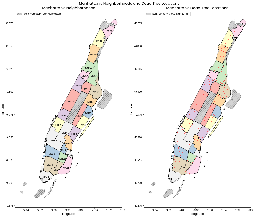
Manhattan's Neighborhoods and Dead Tree Locations
Left: A map of Manhattan's neighborhoods with neighborhood codes labelled.
Right: A map of Manhattan's neighborhoods with red points showing locations of dead trees.
Neighborhood code and tree locations are shown in side by side subplots because having them superimposed on the same plot makes it difficult to see some tree locations.
The grey hatched areas are of the "park-cemetery-etc-Manhattan" neighborhood which does not contain any trees in the data provided.
# SCATTERPLOT ON MAP SHOWING DEAD TREE LOCATIONS =======================
# CREATE CANVAS --------------------------------------------------------
fig, ax = dual_layout(
    suptitle="Manhattan's Neighborhoods and Dead Tree Locations",
    titles=("Manhattan's Neighborhoods", "Manhattan's Dead Tree Locations")
)

# PLOT MAP -------------------------------------------------------------
man[man.nta_name=="park-cemetery-etc-Manhattan"].plot(ax=ax[0], **missing_kwds)
man[man.nta_name=="park-cemetery-etc-Manhattan"].plot(ax=ax[1], **missing_kwds)
man.dropna().plot(ax=ax[0], cmap="Pastel1", edgecolor="black")
man.dropna().plot(ax=ax[1], cmap="Pastel1", edgecolor="black")

sns.scatterplot(data=trees[trees.status=="Dead"], x="longitude", y="latitude", ax=ax[1],
                s=1, alpha=1,
                # hue="status",
                color="red"
                )

# ANNOTATIONS ----------------------------------------------------------
for i, row in man.dropna().iterrows():
    ax[0].annotate(row["ntacode"], xy=row["point"],
        horizontalalignment="center", fontsize=10,
        verticalalignment="top")

# LEGEND ---------------------------------------------------------------
ax[0].legend([AnyObject()], ['park-cemetery-etc-Manhattan'],
           handler_map={AnyObject: AnyObjectHandler()}, loc="upper left")
ax[1].legend([AnyObject()], ['park-cemetery-etc-Manhattan'],
           handler_map={AnyObject: AnyObjectHandler()}, loc="upper left")

# fig.savefig("figs/trees_dead.png", bbox_inches="tight", facecolor="white")
plt.close()
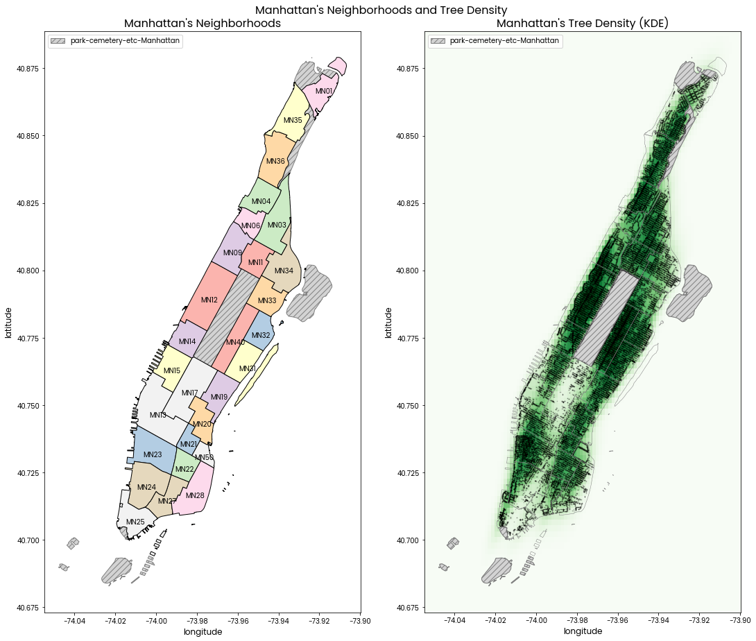
Manhattan's Neighborhoods and Tree Density
Left: A map of Manhattan's neighborhoods with neighborhood codes labelled.
Right: A map of Manhattan's neighborhoods with dark green points showing locations of trees AND a ligher green kernel density estimation of the distribution of trees.
Neighborhood code and tree locations are shown in side by side subplots because having them superimposed on the same plot makes it difficult to see some tree locations.
The grey hatched areas are of the "park-cemetery-etc-Manhattan" neighborhood which does not contain any trees in the data provided.
# KDEPLOT ON MAP SHOWING TREE DENSITY ==================================
# CREATE CANVAS --------------------------------------------------------
fig, ax = dual_layout(
    suptitle="Manhattan's Neighborhoods and Tree Density",
    titles=("Manhattan's Neighborhoods", "Manhattan's Tree Density (KDE)")
)

# PLOT MAP -------------------------------------------------------------
man[man.nta_name=="park-cemetery-etc-Manhattan"].plot(ax=ax[0], **missing_kwds)
man[man.nta_name=="park-cemetery-etc-Manhattan"].plot(ax=ax[1], **missing_kwds)
man.dropna().plot(ax=ax[0], cmap="Pastel1", edgecolor="black")

# COMPUTE KDE ----------------------------------------------------------
try:
    Z # Don't recalculate
except NameError:
    # xmax, ymax = trees[["longitude", "latitude"]].max()
    # xmin, ymin = trees[["longitude", "latitude"]].min()
    xmin, xmax = ax[0].get_xlim()
    ymin, ymax = ax[0].get_ylim()
    X, Y = np.mgrid[xmin:xmax:100j, ymin:ymax:100j]
    positions = np.vstack([X.ravel(), Y.ravel()])
    values = np.vstack([trees["longitude"].values, trees["latitude"].values])
    kernel = stats.gaussian_kde(values)
    Z = np.reshape(kernel(positions).T, X.shape)

# PLOT MAP -------------------------------------------------------------
ax[1].scatter(trees["longitude"].values, trees["latitude"].values,
            s=0.5,
            #   color="darkgreen",
            color="black",
            alpha=0.2)
ax[1].imshow(np.rot90(Z),
             extent=[xmin, xmax, ymin, ymax],
             cmap=plt.cm.Greens)
man.boundary.plot(ax=ax[1], edgecolor="grey", linewidth=0.5)

# ANNOTATIONS ----------------------------------------------------------
for i, row in man.dropna().iterrows():
    ax[0].annotate(row["ntacode"], xy=row["point"],
        horizontalalignment="center", fontsize=10,
        verticalalignment="top")

# LEGEND ---------------------------------------------------------------
ax[0].legend([AnyObject()], ['park-cemetery-etc-Manhattan'],
           handler_map={AnyObject: AnyObjectHandler()}, loc="upper left")
ax[1].legend([AnyObject()], ['park-cemetery-etc-Manhattan'],
           handler_map={AnyObject: AnyObjectHandler()}, loc="upper left")

# fig.savefig("figs/trees_kde.png", bbox_inches="tight", facecolor="white")
plt.close()
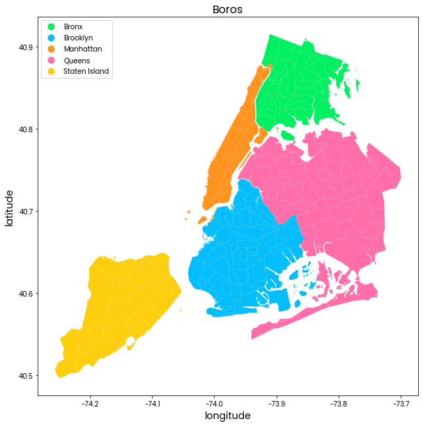
Map: The 5 boros are shown in different colors. The outline of neighborhoods in each boro is shown by a thin white outline.
# PLOT THE BOROS OF NEW YORK ===========================================
fig, ax = plt.subplots(1, 1, figsize=(10, 10))
ax.set_title("Boros", fontsize=16)
ax.set_xlabel("longitude", fontsize=14)
ax.set_ylabel("latitude", fontsize=14)

neighborhoods.plot("boroname", ax=ax,
                   legend=True, legend_kwds={"loc": "upper left"},
                   cmap=src.style.cmap,
                   )
# fig.savefig("figs/boros.png", facecolor="white", bbox_inches="tight")
plt.close()
This can bias our results when trying to determine causes for death.
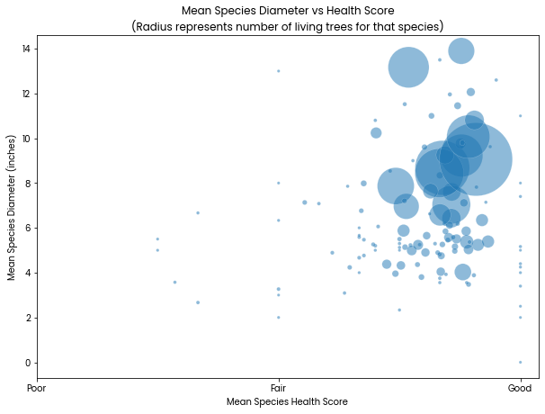
Mean Species Diameter vs Health Score
X: Mean species Health where the categories poor/fair/good are treated as numbers 0/1/2
Y: Mean species diameter in inches measured at 54 inches above the ground
The size of the circles corresponds to how many trees there are of that species. This is only to show that there are more trees (larger circle) for species that tend to be rated healthier and have wider diameter. No species labels are included.
# DIAMETER VS HEALTH ===================================================
# FILTER TO LIVING TREES ONLY ------------------------------------------
df = trees[trees.status == "Alive"].copy()

# HEALTH CATEGORY ->> ORDINAL ------------------------------------------
health_scores = ["Poor", "Fair", "Good"]
df["health"] = df["health"].map(lambda h: health_scores.index(h))

# PER SPECIES AGGREGATES -----------------------------------------------
df = df.groupby("spc_common").agg({
        "spc_common": ["count"],
        "tree_dbh": ["mean", "std"],
        "health": ["mean", "std"],
        "nta": ["nunique"],
    })

# PLOT -----------------------------------------------------------------
fig, ax = plt.subplots(1, 1, figsize=(10, 7))
minsize = df[("spc_common", "count")].min() / 2 + 10
maxsize = df[("spc_common", "count")].max() / 2
sns.scatterplot(
    data=df,
    ax=ax,
    x=("health", "mean"),
    y=("tree_dbh", "mean"),
    alpha=0.5,
    size=("spc_common", "count"), sizes=(minsize, maxsize),
);

ax.set_title("Mean Species Diameter vs Health Score\n(Radius represents number of living trees for that species)")
ax.set_xlabel("Mean Species Health Score")
ax.set_ylabel("Mean Species Diameter (inches)")
ax.set_xticks(range(3));
ax.set_xticklabels(health_scores);
ax.legend().set_visible(False)
# fig.savefig("figs/diameter_vs_health.png", facecolor="white", bbox_inches="tight")
plt.close()